引　言

四象限探测器（four quadrant detector，FQD）是由4个基本相同的光电二极管组成，用来定位外部投射光斑相对四象限探测器中心的位置^[1]。它具有灵敏度高、光谱范围广、位置分辨率高、抗干扰能力强^[2]等优点, 因此常被应用于军事制导、精密检测、航空等领域，并可用于关键部件的力学参数测量，如船用实心轴形变监测、飞机螺旋桨推力测试以及风力发电机转动轴扭矩测量。在利用光学方法测量船用实心轴因海水阻力产生的微小形变时，‌位移、速度或角度参数的测量‌精度均受多种因素影响，‌而光斑中心定位算法的误差是主要误差来源之一。近年来，研究者针对四象限探测器光斑定位精度的影响因素开展了大量研究：文献[3]分析了经典和差算法、对角线算法、对数算法等，但这些算法的测试精度不足；文献[4]提出了高精度的数据库查询法，其仿真误差相对于经典算法的误差显著减小，达到$ {10^{ - 5}} $ mm数量级，但由于计算量大，无法满足实时性需求；文献[5]使用Composite拟合算法进行光斑定位，仿真实验表明，其测量误差为$ {10^{ - 4}} $ mm数量级。该算法是目前应用最广泛的定位算法。以上定位算法都基于标准圆形光斑，这也是目前研究最为广泛的一种模型。文献[6]详细分析了光斑的形状，并建立了椭圆光斑模型。当光束与探测器光敏面法线存在微小夹角时，椭圆光斑模型能够减小由此所产生的误差。但该模型计算光斑中心位置的精度不高，且只讨论了椭圆光斑长短轴与四象限探测器中心坐标系的坐标轴重合这一种情况，并没有分析椭圆光斑长短轴与坐标轴存在偏移角时的情况。

为了解决椭圆光斑长短轴与坐标轴存在偏移角时的定位问题，本研究提出了基于椭圆模型的无穷积分（infinite integral）拟合算法，采用最小二乘法拟合最佳解析表达式。首先进行了仿真计算，该定位算法的测试精度为微米量级，并设计系统对数据进行分析处理。同时，对该算法进行补偿修正，补偿后的精度能够达到亚微米量级，验证了所提方法的有效性。

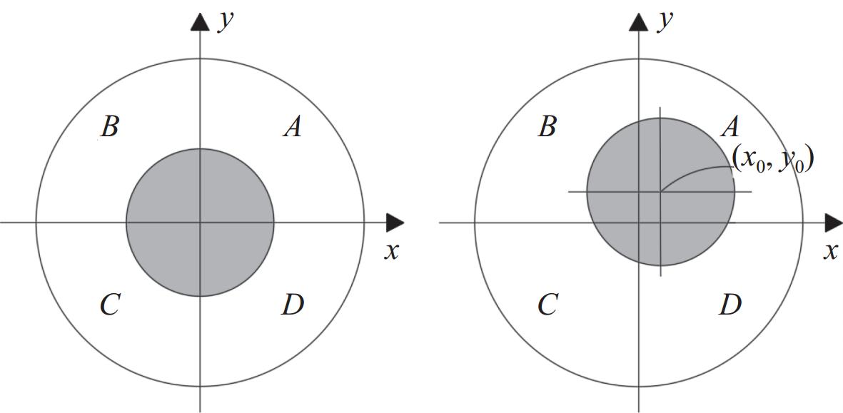
1 四象限探测器光斑定位原理和算法

四象限探测器由4个理论上性能一致的光电二极管组成^[6-7]。如图1所示，4个探测器均匀地排布在直角坐标系的A、B、C、D这 4个象限上。当半导体激光器发出的光束照射在四象限探测器光敏面上时，光电二极管会因受激吸收产生电子，从而形成电流。该电流大小和探测器所接收的光能量成正比^[8]。

当光斑中心$（{x_0}，{y_0}）$相对于四象限探测器光敏面发生偏移时，各象限接收的光能量也会发生变化，从而导致每个光电二极管产生的电流大小发生改变。根据经典的加减法，可以得到光斑中心的解算值$（\mathop x\limits^ \wedge ，\mathop y\limits^ \wedge）$^[6-8]

$ \begin{gathered} \mathop x\limits^ \wedge = \dfrac{{({I_A} + {I_D}) - ({I_B} + {I_C})}}{{{I_A} + {I_B} + {I_C} + {I_D}}} = \dfrac{{({P_A} + {P_D}) - ({P_B} + {P_C})}}{{{P_A} + {P_B} + {P_C} + {P_D}}} \\ \mathop y\limits^ \wedge = \dfrac{{({I_A} + {I_B}) - ({I_C} + {I_D})}}{{{I_A} + {I_B} + {I_C} + {I_D}}} = \dfrac{{({P_A} + {P_B}) - ({P_C} + {P_D})}}{{{P_A} + {P_B} + {P_C} + {P_D}}} \\ \end{gathered} $

(1)

式中：$（\mathop x\limits^ \wedge ，\mathop y\limits^ \wedge ）$为光斑中心在四象限探测器上的解算值；$ {I_A} $、$ {I_B} $、$ {I_C} $、$ {I_D} $为四象限探测器每个象限产生的光电流；$ {P_A} $、$ {P_B} $、$ {P_C} $、$ {P_D} $为每个象限接收的光能量。

2 基于椭圆高斯光斑四象限探测器定位算法 2.1 椭圆高斯光斑模型

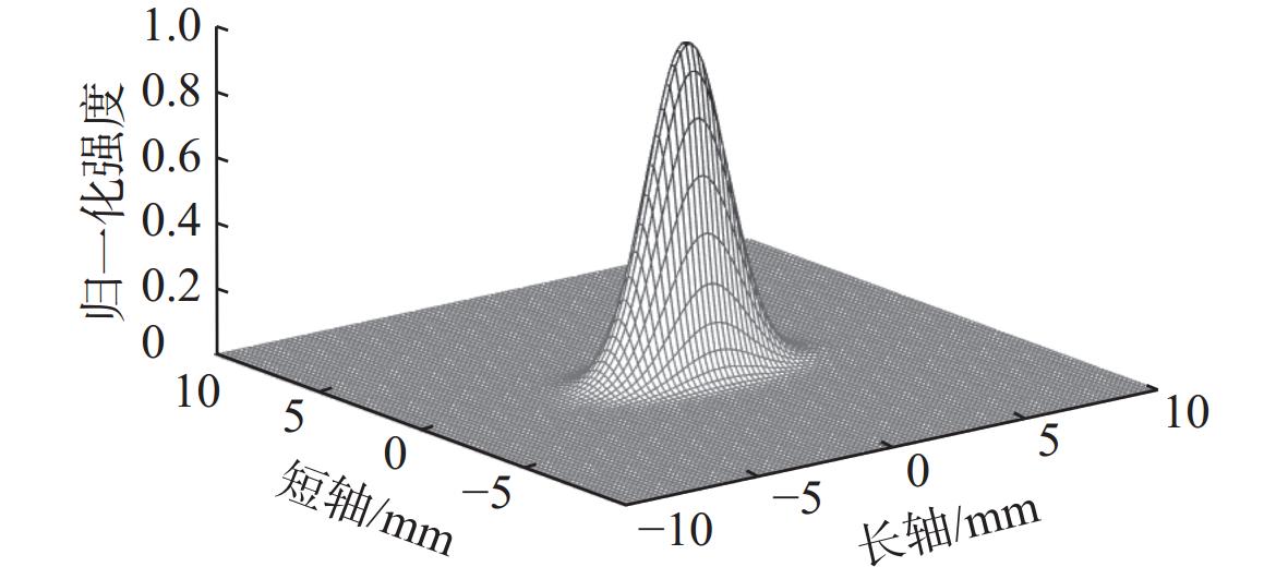
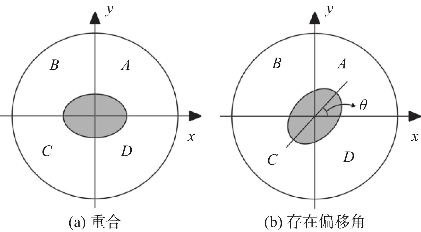
当激光在真空或大气中近距离传输时，照射于四象限探测器光敏面上的光束能量分布可近似为高斯分布^[9]，具有中心强度最高，径向强度逐渐衰减的特征，如图2所示。激光照射光斑的位置情况可以分为两种：一种如图3（a）所示，椭圆光斑长短轴与四象限探测器坐标轴重合；另一种如图3（b）所示，椭圆光斑长短轴与四象限探测器坐标轴存在偏移角。

椭圆高斯光斑的能量分布函数^[10]为

$ {E_{}}(x,y) = \dfrac{{2{I_0}}}{{{\text{π }}{r_x}{r_y}}}\exp \left[ { - \left(\dfrac{{2x_\theta^2}}{{r_x^2}} + \dfrac{{2y_\theta^2}}{{r_y^2}}\right) }\right] $

(2)

其中

$ \begin{gathered} {x_\theta } = (x - {x_0}) \cdot \cos \theta + (y - {y_0}) \cdot \sin \theta \\ {y_\theta } = - (x - {x_0}) \cdot \sin \theta + (y - {y_0}) \cdot \cos \theta \\ \end{gathered} $

(3)

式中：（x，y）为光斑任意点坐标；I₀为高斯光斑总能量；$ {r_x} $、$ {r_y} $为椭圆高斯光斑的长轴和短轴；$ （{x_0}，{y_0}） $为光斑中心坐标；θ为椭圆光斑长短轴相对四象限探测器坐标系x、y轴的偏移角。圆形高斯光斑能量分布也可以用该函数来表示。

2.2 基于椭圆高斯光斑的无穷积分定位算法

根据以上椭圆形光斑能量分布模型，再结合四象限探测器的象限宽度半径R，同时将探测器光敏面的盲区半宽度d考虑在内，通过式（4）可以更加精确地推导出椭圆光斑在四象限探测器各象限的光能量^[11]。

$ \begin{gathered} {P_A} = \displaystyle\int_d^R {\displaystyle\int_d^R {{E_{}}(x,y){\text{d}}x{\text{d}}y} } \\ {P_B} = \displaystyle\int_{ - R}^{ - d} {\displaystyle\int_d^R {{E_{}}(x,y){\text{d}}x{\text{d}}y} } \\ {P_C} = \displaystyle\int_{ - R}^{ - d} {\displaystyle\int_{ - R}^{ - d} {{E_{}}(x,y){\text{d}}x{\text{d}}y} } \\ {P_D} = \displaystyle\int_d^R {\displaystyle\int_{ - R}^{ - d} {{E_{}}(x,y){\text{d}}x{\text{d}}y} } \end{gathered} $

(4)

将式（4）代入式（1），可得到光斑中心位置相对于四象限探测器中心的解算表达式

$ \begin{aligned} \mathop x\limits^ \wedge =&\; \dfrac{{({P_A} + {P_D}) - ({P_B} + {P_C})}}{{{P_A} + {P_B} + {P_C} + {P_D}}} =\\& \dfrac{{\bigg[\displaystyle\int_d^R {\displaystyle\int_d^R {E(x,y){\text{d}}x{\text{d}}y} } + \displaystyle\int_d^R {\displaystyle\int_{ - R}^{ - d} {E(x,y){\text{d}}x{\text{d}}y\bigg]} } - \bigg[\displaystyle\int_{ - R}^{ - d} {\displaystyle\int_d^R {E(x,y){\text{d}}x{\text{d}}y} + } \displaystyle\int_{ - R}^{ - d} {\displaystyle\int_{ - R}^{ - d} {E(x,y){\text{d}}x{\text{d}}y} } \bigg]}}{{\displaystyle\int_d^R {\displaystyle\int_d^R {E(x,y){\text{d}}x{\text{d}}y} } + \displaystyle\int_{ - R}^{ - d} {\displaystyle\int_d^R {E(x,y){\text{d}}x{\text{d}}y} + } \displaystyle\int_{ - R}^{ - d} {\displaystyle\int_{ - R}^{ - d} {E(x,y){\text{d}}x{\text{d}}y} } + \displaystyle\int_d^R {\displaystyle\int_{ - R}^{ - d} {E(x,y){\text{d}}x{\text{d}}y} } }} \\ \mathop y\limits^ \wedge =&\; \dfrac{{({P_A} + {P_B}) - ({P_C} + {P_D})}}{{{P_A} + {P_B} + {P_C} + {P_D}}} =\\& \dfrac{{\bigg[\displaystyle\int_d^R {\displaystyle\int_d^R {E(x,y){\text{d}}x{\text{d}}y} } + \displaystyle\int_{ - R}^{ - d} {\displaystyle\int_d^R {E(x,y){\text{d}}x{\text{d}}y} \bigg]} - \bigg[\displaystyle\int_{ - R}^{ - d} {\displaystyle\int_{ - R}^{ - d} {E(x,y){\text{d}}x{\text{d}}y} } + \displaystyle\int_d^R {\displaystyle\int_{ - R}^{ - d} {E(x,y){\text{d}}x{\text{d}}y} } \bigg]}}{{\displaystyle\int_d^R {\displaystyle\int_d^R {E(x,y){\text{d}}x{\text{d}}y} } + \displaystyle\int_{ - R}^{ - d} {\displaystyle\int_d^R {E(x,y){\text{d}}x{\text{d}}y} + } \displaystyle\int_{ - R}^{ - d} {\displaystyle\int_{ - R}^{ - d} {E(x,y){\text{d}}x{\text{d}}y} } + \displaystyle\int_d^R {\displaystyle\int_{ - R}^{ - d} {E(x,y){\text{d}}x{\text{d}}y} } }} \end{aligned}$

(5)

式（5）属于超越方程，无法求解。高斯光斑在光敏面外的光强很弱，可以忽略不计，将积分的上下限转化成无穷，可以对方程进行求解，得到的表达式为^[12]

$ \begin{gathered} \mathop x\limits^ \wedge = {\text{erf}}\left(\dfrac{{\sqrt 2 }}{{{r_x}}}{x_0}\right) \\ \mathop y\limits^ \wedge = {\text{erf}}\left(\dfrac{{\sqrt 2 }}{{{r_y}}}{y_0}\right) \\ \end{gathered} $

(6)

式中，$ {\text{erf}}(\alpha ) = \dfrac{2}{{\sqrt {\text{π }} }}\displaystyle\int_0^\alpha {{{\text{e}}^{ - {t ^2}}}{\text{d}}t} $，为误差函数，其中t为积分运算的中间变量。对式（6）两边取反函数，可得到关于$ \mathop x\limits^ \wedge $和$ \mathop y\limits^ \wedge $的近似解。

同理，x₀和y₀的表达式为

$ \begin{gathered} {x_0} = \dfrac{{{\text{er}}{{\text{f}}^{ - 1}}(\mathop x\limits^ \wedge ){r_x}}}{{\sqrt 2 }} \\ {y_0} = \dfrac{{{\text{er}}{{\text{f}}^{ - 1}}(\mathop y\limits^ \wedge ){r_y}}}{{\sqrt 2 }} \\ \end{gathered} $

(7)

可将式（7）中的光斑中心位置近似表达式改写为

$ \begin{gathered} {x_0} = \dfrac{{{\text{er}}{{\text{f}}^{ - 1}}(\mathop x\limits^ \wedge ){r_x}}}{{\sqrt 2 }} = g(\mathop x\limits^ \wedge ) \times {r_x} \\ {y_0} = \dfrac{{{\text{er}}{{\text{f}}^{ - 1}}(\mathop y\limits^ \wedge ){r_x}}}{{\sqrt 2 }} = g(\mathop y\limits^ \wedge ) \times {r_y} \\ \end{gathered} $

(8)

式中，$ g(\mathop x\limits^ \wedge ) = {\text{er}}{{\text{f}}^{ - 1}}(\mathop x\limits^ \wedge )/\sqrt 2 $，是仅关于$ \mathop x\limits^ \wedge $的函数，可通过查表得到。但它未考虑四象限探测器光敏面外环境的影响，所以其误差较大。为了提高四象限探测器检测精度和线性检测范围，引入补偿因子^[13]$ \eta $对行函数进行拟合。光斑中心位置的解析表达式为

$ \begin{gathered} {x_\theta } = g(\mathop x\limits^ \wedge ) \times {r_x} \times {\eta _x}({r_x},R,d,\theta ) \\ {y_\theta } = g(\mathop y\limits^ \wedge ) \times {r_y} \times {\eta _y}({r_y},R,d,\theta ) \\ \end{gathered} $

(9)

在$ \eta $中引入影响因素 $ {r_x} $、$ {r_y} $，可将式（9）后两项合并，得

$ \begin{gathered} {x_\theta } = g(\mathop x\limits^ \wedge ) \times {\eta _x}({r_x},R,d,\theta ) \\ {y_\theta } = g(\mathop y\limits^ \wedge ) \times {\eta _y}({r_y},R,d,\theta ) \\ \end{gathered} $

(10)

为了得到补偿因子$ {\eta _x}、{\eta _y} $的函数，假设椭圆高斯光斑照射在半径为R，盲区宽度为2d的四象限探测器光敏面上。将光斑中心$ （X{}_i，{Y_i}） $从$ （- \mu ，0） $移动到$ （\mu ，0） $，步长为$ {\sigma _{\mathrm{s}}} $，记录每一步中四象限输出电流值，将真实值$ （X{}_i，{Y_i}） $和解算值$ （\mathop x\limits^ \wedge ，\mathop y\limits^ \wedge ） $一一映射。采用最小二乘法，建立位置检测误差的数学模型

$ \begin{gathered} I({\eta _x}) = {\| {{{\text{δ}}_x}} \|^2} = \displaystyle\sum\limits_{i = 1}^N {\left[ {x(\mathop x\limits^ \wedge ,{\eta _x}) - {X_i}} \right]} \\ I({\eta _y}) = {\| {{{\text{δ}}_y}} \|^2} = \displaystyle\sum\limits_{i = 1}^N {\left[ {y(\mathop y\limits^ \wedge ,{\eta _y}) - {Y_i}} \right]} \\ \end{gathered} $

(11)

对等式两边求导，得到

$ \begin{gathered} \dfrac{{\partial I}}{{\partial {\eta _x}}} = 2\displaystyle\sum\limits_{i = 1}^N {{g^2}(\mathop x\limits^ \wedge )} \times {\eta _x} - 2\displaystyle\sum\limits_{i = 1}^N {g(\mathop x\limits^ \wedge )} \times {X_i} \\ \dfrac{{\partial I}}{{\partial {\eta _y}}} = 2\displaystyle\sum\limits_{i = 1}^N {{g^2}(\mathop y\limits^ \wedge )} \times {\eta _y} - 2\displaystyle\sum\limits_{i = 1}^N {g(\mathop y\limits^ \wedge )} \times {Y_i} \\ \end{gathered} $

(12)

令$ \dfrac{{\partial I}}{{\partial {\eta _{x,y}}}} $= 0，计算出最优$ {\eta _x}、{\eta _y} $

$ {\eta _x} = \dfrac{{\displaystyle\sum\limits_{i = 1}^N {g(\mathop x\limits^ \wedge )} \times {X_i}}}{{\displaystyle\sum\limits_{i = 1}^N {{g^2}(\mathop x\limits^ \wedge )} }},\;\;{\eta _y} = \dfrac{{\displaystyle\sum\limits_{i = 1}^N {g(\mathop y\limits^ \wedge )} \times {Y_i}}}{{\displaystyle\sum\limits_{i = 1}^N {{g^2}(\mathop y\limits^ \wedge )} }} $

(13)

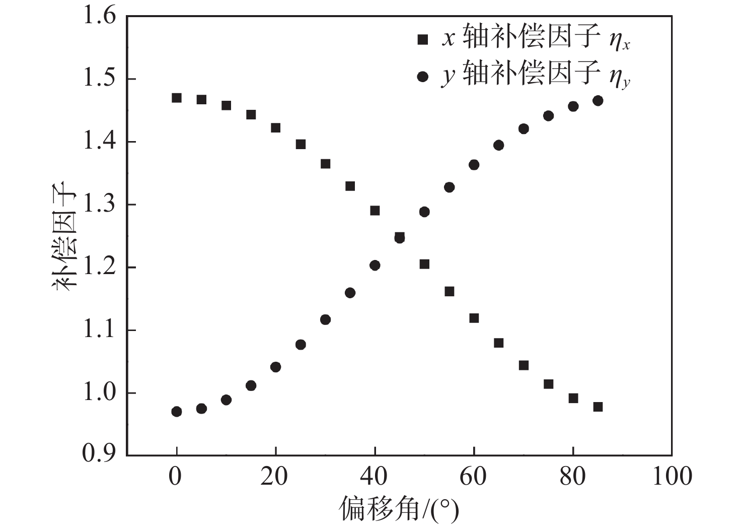
本文以R = 3.8 mm，d = 0.021 mm的四象限探测器为例进行仿真分析，该定位算法也适用于其他四象限探测器。在实际应用中，选定好合适的四象限探测器和光源后，保持探测器和光源的距离不变，就可将测量系统中四象限探测器的R、d和光斑的$ {r_x} $、$ {r_y} $视为固定值。当入射光斑的长短轴分别为3 mm和2 mm时，设定不同偏移角$ \theta $，则补偿因子$ {\eta _x}、{\eta _y} $是仅关于$ \theta $的函数。由图4可知，长轴与四象限探测器坐标系中x轴重合，短轴与y轴重合的椭圆光斑绕中心点逆时针旋转时，长短轴与四象限探测器坐标轴的偏移角将越来越大，x轴的补偿因子会随之减小，而y轴的补偿因子会随之增大。

由图4可知，补偿因子$ {\eta _x}、{\eta _y} $是关于$ \theta $的函数，通过五次多项式进行拟合，计算式为

$ \;\begin{aligned} & {\eta _x} = 1.470 \;2 - 1.268 \;53 \times {10^{ - 4}} \times \theta - 1.043\; 73 \times {10^{ - 4}} \times\\ &\;\; {\theta ^2} - 7.738 \;96 \times {10^{ - 7}} \times {\theta ^3} + 1.801 \;7 \times {10^{ - 8}} \times {\theta ^4} - \\ &\;\; 4.336\; 46 \times {10^{ - 11}} \times {\theta ^5} \\ &{\eta _y} = 0.970 \;53 - 2.331 \;88 \times {10^{ - 4}} \times \theta + 2.243\; 8 \times {10^{ - 4}} \times \\ &\;\; {\theta ^2} - 1.598\; 69 \times {10^{ - 6}} \times {\theta ^3} - 8.841 \;77 \times {10^{ - 9}} \times {\theta ^4} + \\ &\;\; 7.597\; 71 \times {10^{ - 11}} \times {\theta ^5} \end{aligned}$

(14)

在其他因素都确定的情况下，根据四象限探测器输出的$ （\mathop x\limits^ \wedge ，\mathop y\limits^ \wedge ） $，及式（14）求出的补偿因子就可求出光斑中心位置$ （{x_\theta }，{y_\theta }） $，其拟合表达式为

$ \begin{aligned} {x}_\theta=& {g}(\stackrel{\wedge }{x})\times (1.470\;2-1.268\;53\times {10}^{-4}\times \theta -\\ & 1.043\;73 \times {10}^{-4} \times {\theta }^{2} - 7.738\;96 \times {10}^{-7}\times {\theta }^{3} +\\ & 1.801\;7 \times {10}^{-8} \times {\theta }^{4}-4.336\;46\times {10}^{-11}\times {\theta }^{5})\\ {y}_\theta=& {g}(\stackrel{\wedge }{y})\times (0.970\;53-2.331\;88\times {10}^{-4}\times \theta +\\ & 2.243\;8 \times {10}^{-4} \times {\theta }^{2} - 1.598\;69\times {10}^{-6}\times {\theta }^{3} -\\ & 8.841\;77 \times {10}^{-9} \times {\theta }^{4} + 7.597\;71 \times {10}^{-11}\times {\theta }^{5}) \end{aligned}$

(15)

由式（15）可知，对于同一套测试系统，在四象限探测器和光源确定的情况下，只需做一组标定实验就可以确定光斑中心位置与偏移角的关系。这不仅能减少计算量，还能使定位精度达到微米量级。

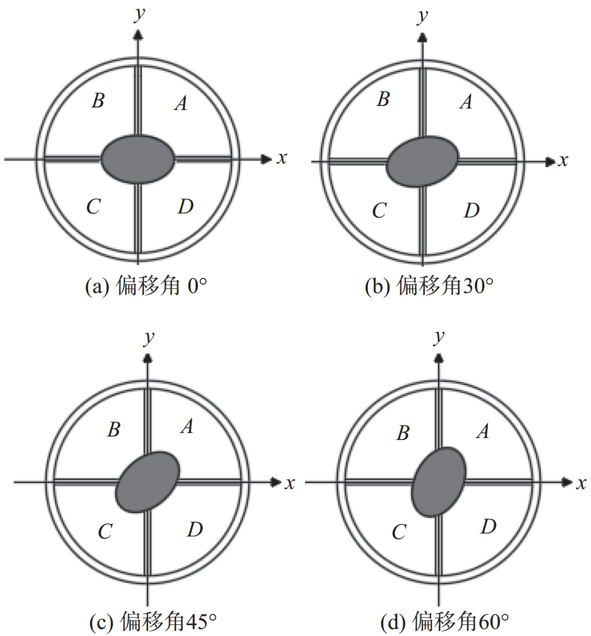
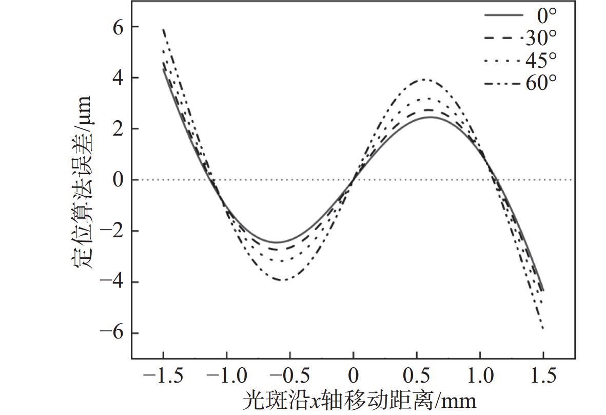
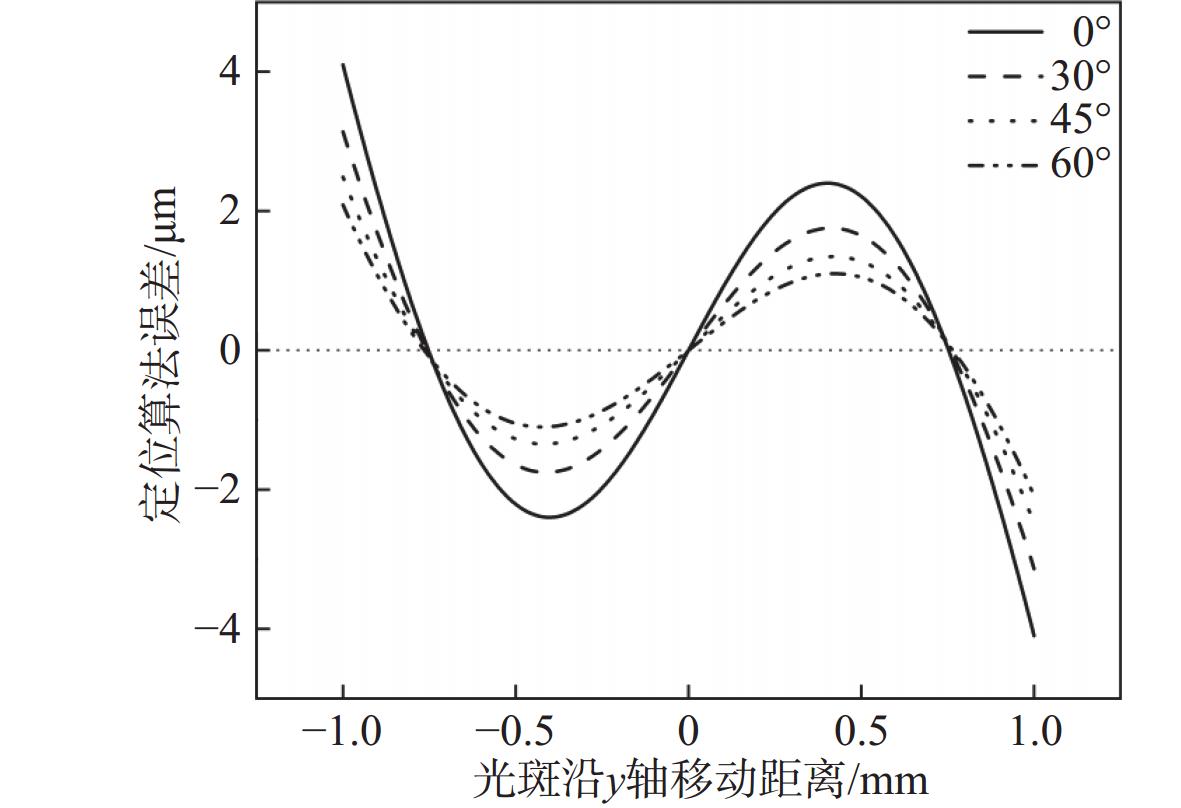
仿真计算了偏移角分别为0°、30°、45°和60°（见图5）时，椭圆光斑沿x或y轴移动时的定位算法误差。图6所示为，椭圆光斑沿x轴移动时的定位算法误差。由图可知，当偏移角分别为0°、30°、45°和60°时，4条误差曲线均关于原点对称，且x轴的定位算法误差及最大误差值均随偏移角的增大而增大。在（0，0.75） mm区间内，定位算法误差随偏移角增大而增大。图7是椭圆光斑沿y轴移动时的定位算法误差，曲线的变化趋势与x轴的相同，但在（0，0.5） mm区间内，y轴的定位算法误差随偏移角的增大而逐渐减小。

3 实验与结果分析

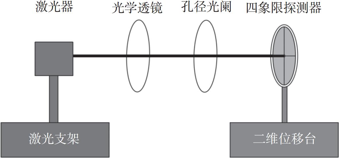
为了验证椭圆光斑模型无穷积分拟合算法的有效性和精度，设计了基于四象限探测器的光斑位置检测系统。它包括波长为620 nm的激光器，直径为7.8 mm的光敏面，盲区为0.042 mm的四象限探测器（Thorlabs，QPD80A）以及二维精密位移台。系统还包括信号采集和数据处理模块，其中采集卡（VKINGING，VK702N）的本底噪声为0.12 mV。图8为检测系统示意图，激光器发出的光束经光学透镜和孔径光阑后，形成长轴为3mm，短轴为2 mm的椭圆光斑测试光束。将四象限探测器固定安装于微米级二维位移台上，可实现x、y轴方向的精密移动。

仿真验证了基于椭圆高斯光斑的定位算法。采用图8所示实验平台，通过手动旋转平台（最小刻度为10′）调整角度，当椭圆光斑长轴与四象限探测器光敏面坐标系x轴呈0°、30°、45°和60°夹角时，进行了光斑长轴和短轴的标定实验。将光斑中心从（−1 mm，0）移动到（1 mm，0），步长为10 μm，在每个位移点采集四象限探测器的输出电流值。通过式（1）的解算位移值和真实位移值建立映射关系，标定光斑x轴补偿因子。y轴补偿因子则通过二维位移台将光斑中心从（0，−0.8 mm）移动到（0，0.8 mm），步长为10 μm，进行算法标定。接着，将光斑中心从（−1 mm，0）移动到（1 mm，0），从（0，−0.8 mm）移动到（0，0.8 mm），步长为20 μm，在每个位移点采集四象限探测器的输出电流值。利用输出电流值及标定实验获得的补偿因子定位光斑位置。将定位算法的计算结果与光斑真实位置进行比对，以验证算法的定位精度。

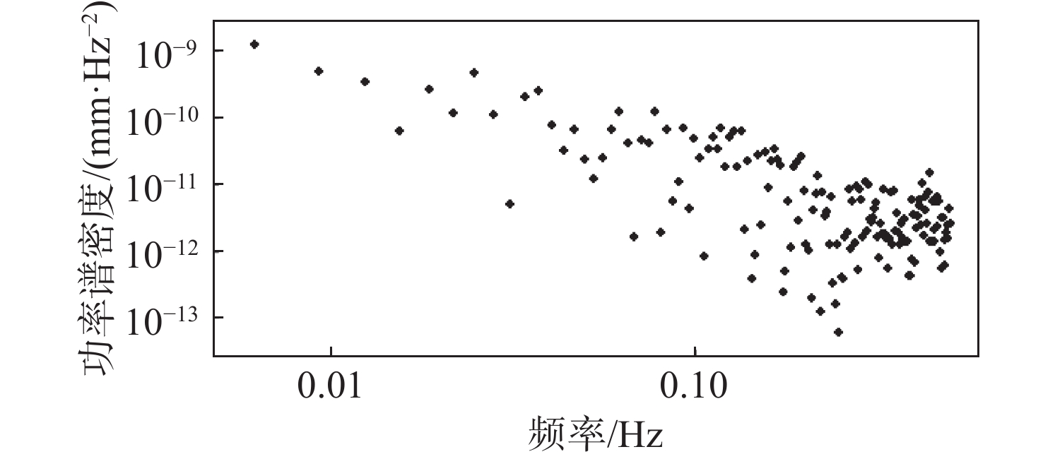
图9所示为静态遮光条件下，测试系统的四象限探测器输出功率谱密度，采集卡的采集频率为1 Hz。在采集范围内，测得系统最大噪声为$ 3.79 \times {10^{ - 5}} $ mm。

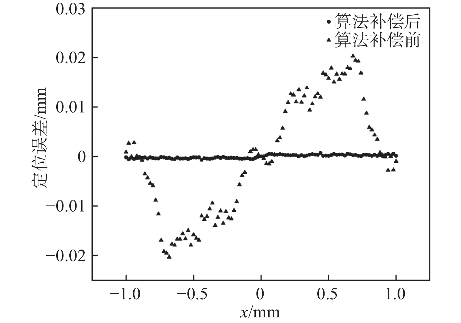
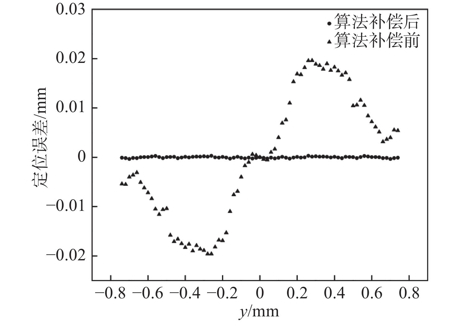
图10所示为偏移角为45°时x轴定位算法补偿前后的误差曲线，图中小三角形标识曲线为定位算法计算值与真实值之间的误差。由图6和图7所示仿真结果可知，定位误差曲线在负半轴和正半轴呈对称，所以本文主要分析正半轴区间（0，1） mm内定位算法的误差，并采用均方根误差（root mean squared error，RMSE）E_rms来描述定位精度。$ {E_{{\text{rms}}}} = \sqrt {\dfrac{1}{N}{{\displaystyle\sum\limits_{i = 1}^N {\left( {{X_i} - X} \right)} ^2}}} $，N为定位次数，$ {X_i} $为光斑定位算法计算值，X为光斑移动真实值。在（0，1） mm区间内，补偿前定位算法x轴的E_rms为8.159 5 μm。由图6可知，偏移角为45°时，仿真计算x轴的E_rms为2.375 μm。定位算法误差曲线的变化趋势和仿真结果大体相同，验证了本文算法的可行性。补偿前算法的固定误差为微米量级，为提高光斑定位精度，需对标定实验得出的误差值进行补偿。图10中小圆点标识的为补偿后x轴误差曲线，其E_rms为0.219 3 μm，相对于补偿前算法精度提高了97.3%。同理，图11为y轴定位算法补偿前后的误差曲线，图中小三角形标识曲线为定位算法计算值与真实值之间的误差。在（0，0.75） mm区间内，定位算法误差曲线趋势与图7所示仿真结果相似，验证了椭圆无穷积分算法的可行性。补偿前定位算法y轴的E_rms为7.019 2 μm。由图7可知，偏移角为45°时，仿真计算y轴的E_rms为0.964 μm。图11中小圆点标识的为补偿后y轴误差曲线，其E_rms为0.267 6 μm，相对于补偿前的算法精度提高了96.2%。理论上，修正后的E_rms应该为0，但由于系统处于光照不稳定环境，杂光进入等原因会使得系统噪声误差增大。在静态遮光条件下，系统最大噪声误差为3.79 ×10⁻⁵ mm，所以补偿后的误差精度为亚微米量级，x轴和y轴的测量精度已经达到了船用轴承形变量测量标准^[14]。

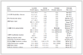
表1所示为不同偏移角时，补偿前后定位算法的均方根误差。由结果可知，在x轴方向偏移角越大，均方根误差越大；在y轴方向，偏移角越大，均方根误差越小。这与图6和图7所示仿真结果相同。本文提出的椭圆无穷积分算法在补偿后，x轴和y轴方向的E_rms相对于补偿前降低了94.83%～97.80%。

4 结　论

本文提出基于椭圆高斯模型的无穷积分拟合定位算法，通过仿真计算椭圆光斑长短轴与探测器坐标系坐标轴间的偏移角，验证了算法对任意偏移角度的适应性；在固定光源与四象限探测器的条件下，通过标定实验建立了光斑中心坐标关于偏移角的函数模型；进一步通过补偿修正将检测精度提升至10^－4 mm，满足船用轴承形变测试精度。未来在椭圆光斑定位精度的研究中需对信号放大处理电路^[15]进行重点讨论，因为在小信号的处理过程中电磁干扰会显著降低定位精度，优化算法和抗干扰设计是后续的核心研究方向。