 2022, Vol. 44
 Issue (6): 36-43


光子可以携带与偏振态有关的自旋角动量(SAM)和与螺旋相位有关的轨道角动量(OAM)[1]。在被广泛研究的空间域涡旋光束中,其携带的纵向OAM与光束的传播方向平行,并且只能在光束横截面内观察到涡旋相位。涡旋结构与光子轨道角动量密切相关[2-4],这在光学及量子信息通信技术中得到验证。如Mair等[5]演示了携带OAM的电磁场空间模型,Uchida等[6]报道了自由空间中携带OAM的电子束的产生,Wang等[7]的研究表明在通信领域OAM可能是提高自由空间通信能力的一个有用的自由度,Bozinovic等[8]演示了利用光的轨道角动量来建立不同的数据传输通道的可能性。
随着对涡旋光束的研究越来越深入,时空域光涡旋(STOV)引起了人们的极大兴趣。通过引入时间域内的相位变化,所形成的涡旋光束绕着垂直于传播方向的轴旋转,可以获得纯横向OAM。在时空光场领域一些关于时空光涡旋和横向OAM的开创性研究已经发表,比如Bliokh等[9]在理论上构造出可以任意角度携带轨道角动量的波束,Jhajj等[10]从实验上证实时空光涡旋的存在,Hancock等[11]演示了时空光涡旋在自由空间中的产生和传播,Chong[12]利用空间频率-频率面到空间-时间面的傅里叶变化,成功生成并表征了携带横向OAM的超短脉冲光波包。
在之前的研究中,我们已经使用预处理的时空波包,在焦平面处产生具有横向OAM的标量STOV[13]。本文主要介绍强聚焦条件下生成偏振态可控的线偏振时空光涡旋的方法,并对聚焦后的波包性质进行分析。该方法为实验生成高度局域的矢量时空光涡旋铺平了道路,在纳米光子学、光与物质相互作用、电光镊等方面具有潜在的应用前景。
1 入射波包预处理不失一般性,具有拉盖尔-高斯模分布且拓扑荷为+1的水平偏振STOV可表述为
| $ {{\boldsymbol{E}}_{ + 1}}(x,y,t) = \left( {\begin{array}{*{20}{c}} {{{\boldsymbol{e}}_x}} \\ 0 \end{array}} \right)\left( {x + {\rm{i}}}t \right)\exp \left( { - \frac{{{x^2} + {y^2}}}{{{\omega ^2}}} - \frac{{{t^2}}}{{\omega _t^2}}} \right) $ | (1) |
式中:
| $ {{\boldsymbol{E}}_{ - 1}}(x,y,t) = \left( {\begin{array}{*{20}{c}} {{{\boldsymbol{e}}_x}} \\ 0 \end{array}} \right)\left( {x - {\rm{i}}}t \right)\exp \left( { - \frac{{{x^2} + {y^2}}}{{{\omega ^2}}} - \frac{{{t^2}}}{{\omega _t^2}}} \right) $ | (2) |
通过之前的研究可知,由于时空像散效应,波包中的时空螺旋相位在通过高数值孔径透镜聚焦时会被破坏[13]。为了防止时空相位结构的崩溃,我们用类似于柱透镜模式转换器中用于从厄米–高斯(HG)模式转换为拉盖尔–高斯(LG)模式的预处理方式,以此来产生强聚焦时空光涡旋波包[14]。由于HG模式可以由LG模式线性叠加而成,上述两个水平线偏振时空光涡旋波包线性叠加之后可获得所需的预劈裂入射时空波包:
| $ \begin{split} {\boldsymbol{E}}_x^{ + 1}\left( {x,y,t} \right) =& {{\boldsymbol{E}}_{ + 1}}\left( {x,y,t} \right) + {\rm{i}}{{\boldsymbol{E}}_{ - 1}}\left( {x,y,t} \right) \\ =& \left( {\begin{array}{*{20}{c}} {{{\boldsymbol{e}}_x}} \\ 0 \end{array}} \right)\left( {1 + {\rm{i}}} \right)\left( {x + t} \right)\exp \left( { - \frac{{{x^2} + {y^2}}}{{{\omega ^2}}} - \frac{{{t^2}}}{{\omega _t^2}}} \right) \end{split} $ | (3) |
类似地,垂直线偏振入射场和45°偏振入射场分别为
| $ {\boldsymbol{E}}_y^{ + 1}\left( {x,y,t} \right) = \left( {\begin{array}{*{20}{c}} 0 \\ {{{\boldsymbol{e}}_y}} \end{array}} \right)\left( {1 + {\rm{i}}} \right)\left( {x + t} \right)\exp \left( { - \frac{{{x^2} + {y^2}}}{{{\omega ^2}}} - \frac{{{t^2}}}{{\omega _t^2}}} \right) $ | (4) |
式中
| $ {\boldsymbol{E}}_{xy}^{ + 1}\left( {x,y,t} \right) = \left( {\begin{array}{*{20}{c}} {{{\boldsymbol{e}}_x}} \\ {{{\boldsymbol{e}}_y}} \end{array}} \right)\left( {1 + {\rm{i}}} \right)\left( {x + t} \right)\exp \left( { - \frac{{{x^2} + {y^2}}}{{{\omega ^2}}} - \frac{{{t^2}}}{{\omega _t^2}}} \right) $ | (5) |
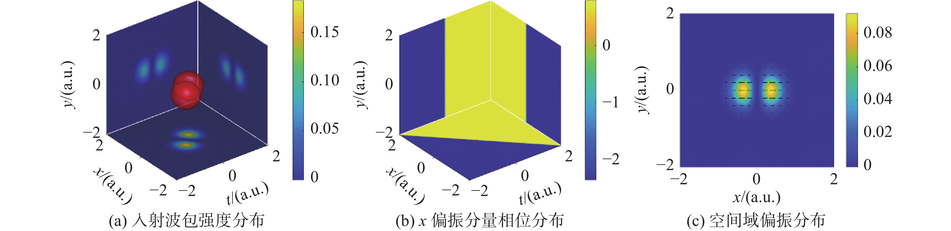
预处理后的水平线偏振入射波包(等值面为峰值强度的10%)如图1(a)所示。从式(3)可知,水平偏振光的y偏振分量为0,因此x偏振分量也就是总入射场,从图1(a)可以看到x偏振分量波包被劈裂成两部分,x=0、y=0、t=0三个截面上的强度分布形状与HG01模相似。如图1(b)所示,x分量的相位分布被二值化为π/4(黄色区域)和−3π/4(蓝色区域)。从图1(c)可以清楚地看出预处理后的波包在空间域为水平线偏振。
|
图 1 水平线偏振入射波包强度、相位及x−y面偏振分布图 Figure 1 Intensity, phase and polarization distribution in x−y plane of horizontally polarized incident wave packet |
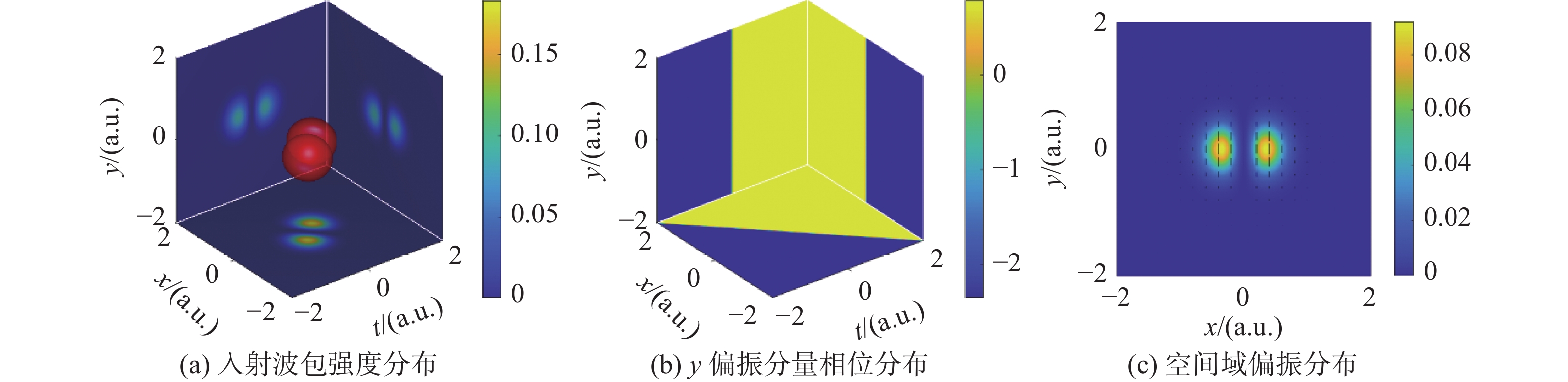
图2为垂直线偏振入射波包强度、相位、偏振分布图。对比图1可以看出,垂直线偏振入射波包形状、强度、相位分布都与水平偏振相同,但空间域偏振分布二者为正交关系。从图2(c)可以看出预处理后的波包在空间域为垂直线偏振。
|
图 2 垂直线偏振入射波包强度、相位及x−y面偏振分布图 Figure 2 Intensity, phase and polarization distribution in x−y plane of vertically polarized incident wave packet |
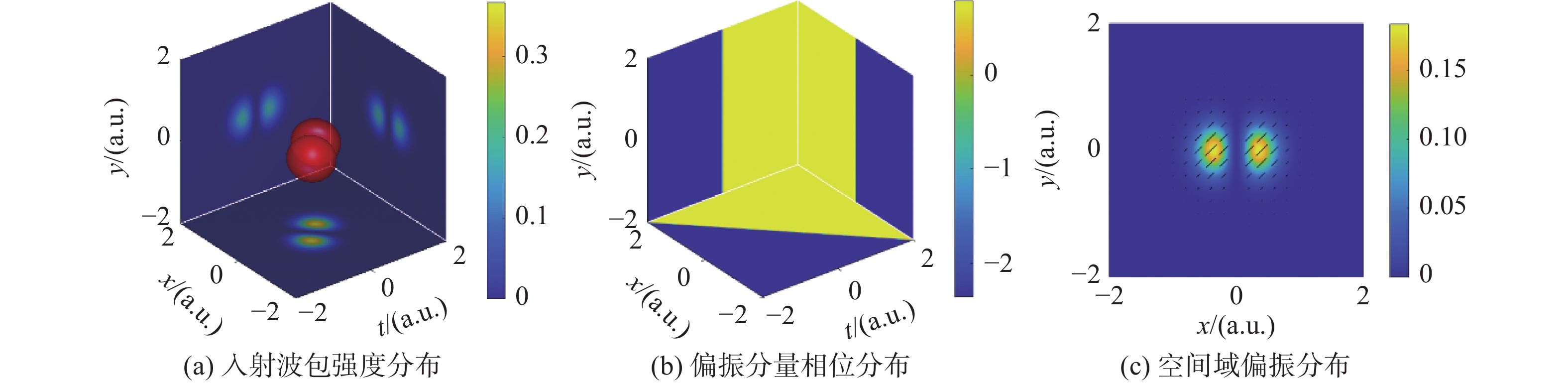
图3为45°线偏振入射波包强度、相位、偏振分布图。从式(5)可知45°线偏振入射波包的x偏振分量和y偏振分量相等。图3(b)反映出45°线偏振入射波包的相位分布与前面的水平、垂直线偏振入射波包的相位分布相同。图3(c)显示预处理后的波包在空间域为45°线偏振。
|
图 3 45°线偏振入射波包强度、相位及x−y面偏振分布图 Figure 3 Intensity, phase and polarization distribution in x−y plane of 45° polarized incident wave packet |
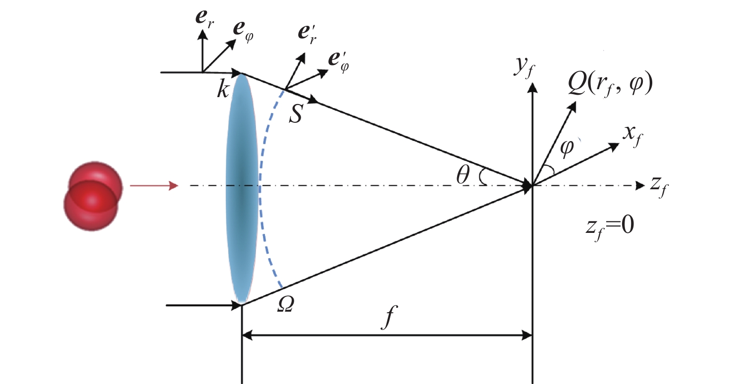
图4给出了预处理波包的强聚焦示意图。其中
|
图 4 时空涡旋强聚焦示意图 Figure 4 Schematic diagram of the tight focusing of STOV |
在后续的模拟仿真中,使用各向同性介质的物镜,将入射波包的空间大小归一化为透镜的NA,设置
在焦场的数值仿真计算中,采用了一种简化的模型,忽略时空耦合,假设入射波包的每个时间切片都聚焦在焦场的共轭位置,同时忽略色差和其它像差的影响。随后利用Debye衍射积分公式计算焦平面上的强聚焦时空波包[15-16]。衍射积分公式如下:
| $ \begin{split} {{\boldsymbol{E}}_f}\left( {{r_f},\varPhi ,{z_f},t} \right) =& \int_0^\alpha {\int_0^{2{\text{π}} } {{\boldsymbol{P}}\left( {\theta ,\phi } \right)B\left( \theta \right)} } {E_\varOmega }\left( {\theta ,\phi ,t} \right) \times \\ & \exp \left\{ - {\rm{i}}k\left[ {r_f}\sin \theta \cos \left( {\phi - \Phi } \right) + \right. \right.\\ & \left. \left.{z_f}\cos \theta \right] \right\}\sin \theta {\rm{d}}\theta {\rm{d}}\phi \end{split}$ | (6) |
式中α是由透镜的NA决定的收敛半角。
| $ {E_\varOmega }\left( {\theta ,\phi ,t} \right) = \left( {1 + {\text{i}}} \right)\left( {\sin \theta \sin \phi + t} \right)\exp \left( { - \frac{{{{\sin }^2}\theta }}{{{\omega ^2}}} - \frac{{{t^2}}}{{\omega _t^2}}} \right) $ | (7) |
水平线偏振光
| $ {\boldsymbol{P}}\left( {\theta ,\phi } \right) = \left( {\begin{array}{*{20}{c}} {\left( {\cos \theta {{\cos }^2}\phi + {{\sin }^2}\phi } \right) \cdot {{{\boldsymbol{e}}'_{{x}}}}} \\ {\left( {\cos \theta \cos \phi \sin \phi - \sin \phi \cos \phi } \right) \cdot {{{\boldsymbol{e}}'_{{y}}}}} \\ {\left( { - \sin \theta \cos \phi } \right) \cdot {{{\boldsymbol{e}}'_{{z}}}}} \end{array}} \right) $ | (8) |
垂直线偏振光
| $ {\boldsymbol{P}}\left( {\theta ,\phi } \right) = \left( {\begin{array}{*{20}{c}} {\left( {\cos \theta \cos \phi \sin \phi - \cos \phi \sin \phi } \right) \cdot {{{\boldsymbol{e}}'_{{x}}}}} \\ {\left( {\cos \theta {{\sin }^2}\phi + {{\cos }^2}\phi } \right) \cdot {{{\boldsymbol{e}}'_{{y}}}}} \\ {\left( { - \sin \theta \sin \phi } \right) \cdot {{{\boldsymbol{e}}'_{{z}}}}} \end{array}} \right) $ | (9) |
45°线偏振光
| $ \begin{split} &{\boldsymbol{P}}\left( {\theta ,\phi } \right) = \\ &\left( {\begin{array}{*{20}{c}} {\left[ {\cos \theta \cos \phi (\sin \phi + \cos \phi ) + \sin \phi (\sin \phi - \cos \phi )} \right] \cdot {{{\boldsymbol{e}}'_{{x}}}}} \\ {\left[ {\cos \theta \sin \phi (\cos \phi + \sin \phi ) + \cos \phi (\cos \phi - \sin \phi )} \right] \cdot {{{\boldsymbol{e}}'_{{y}}}}} \\ {\left[ { - \sin \theta (\sin \phi + \cos \phi )} \right] \cdot {{{\boldsymbol{e}}'_{{z}}}} } \end{array}} \right) \end{split} $ | (10) |
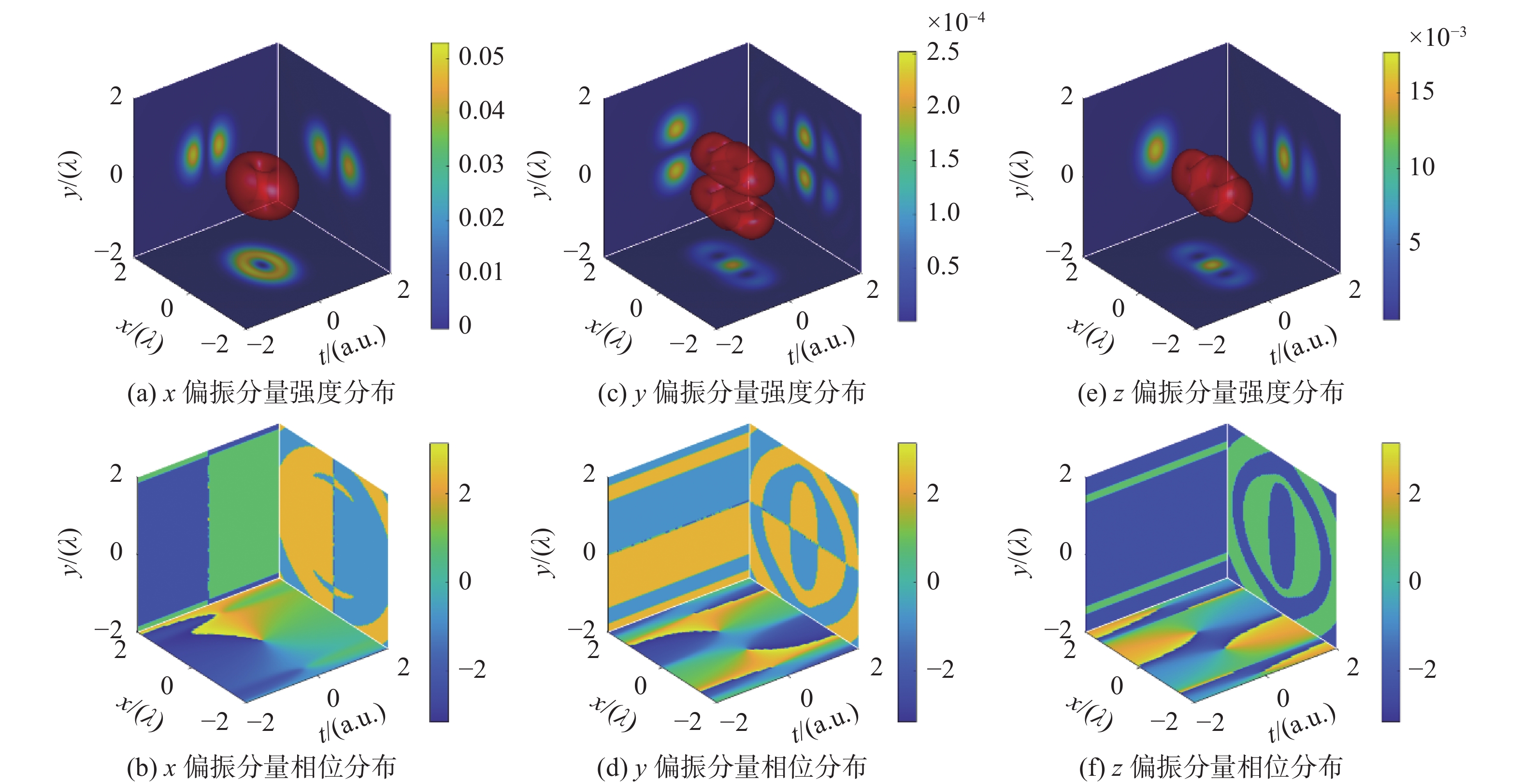
首先,图5给出了水平线偏振入射波包聚焦后焦场的x、y和z偏振分量的强度、相位以及等值面波包图(等值面为最大强度的20%)。图5(a)、5(b)分别是x分量的强度和相位分布图;图5(c)、5(d) 分别是y分量的强度和相位分布图;图5(e)、5(f) 分别是z分量的强度和相位分布图。从图5(a)可以看到等值面波包有一个沿y轴的相位奇点轨迹,对应的相位分布图5(b)在x−t面从−π到π呈逆时针变化,这表明x分量在x−t面内携带拓扑荷+1的横向OAM。从图5(c)可以看到y分量强度很小,和x分量相差2个数量级,因此y分量可以忽略不计。从图5(e)可以看出,聚焦时空涡旋具有较强的z分量,其峰值强度约为x分量的29%。从图5(d)和5(f)可以看到y分量和z分量均沿y轴有两个相位奇点轨迹,相位分布同样从−π到π呈逆时针变化,表明y和z分量在x−t面同时携带两个拓扑荷为+1的横向OAM。
|
图 5 水平线偏振焦场分量强度及相位图 Figure 5 Intensity and phase distribution of the horizontally polarized focal field component |
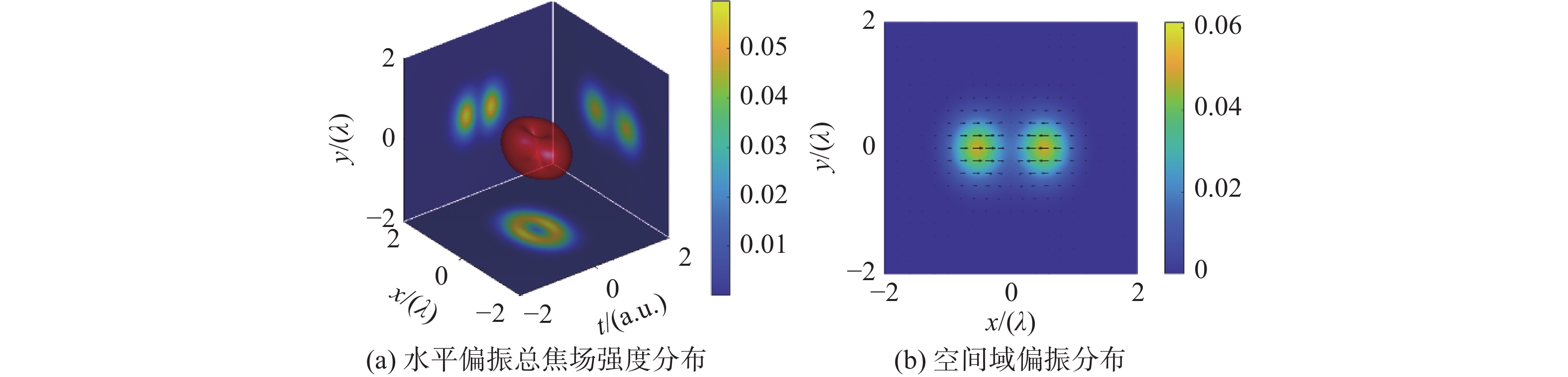
图6给出了聚焦时空涡旋的总强度和偏振分布。图6(a)为聚焦时空涡旋的强度分布及等值面波包图(等值面为最大强度的30%)。总焦场的波包形状与x分量的波包形状基本一致,因此x分量决定了总焦场的波包形状。图6(b)为空间域(x−y面)偏振分布图,从中可以看出聚焦波包在空间域的偏振分布呈水平线偏振。
|
图 6 水平线偏振总焦场强度及x−y面偏振分布图 Figure 6 Total intensity and polarization distribution in x−y plane of the horizontally polarized focused STOV |
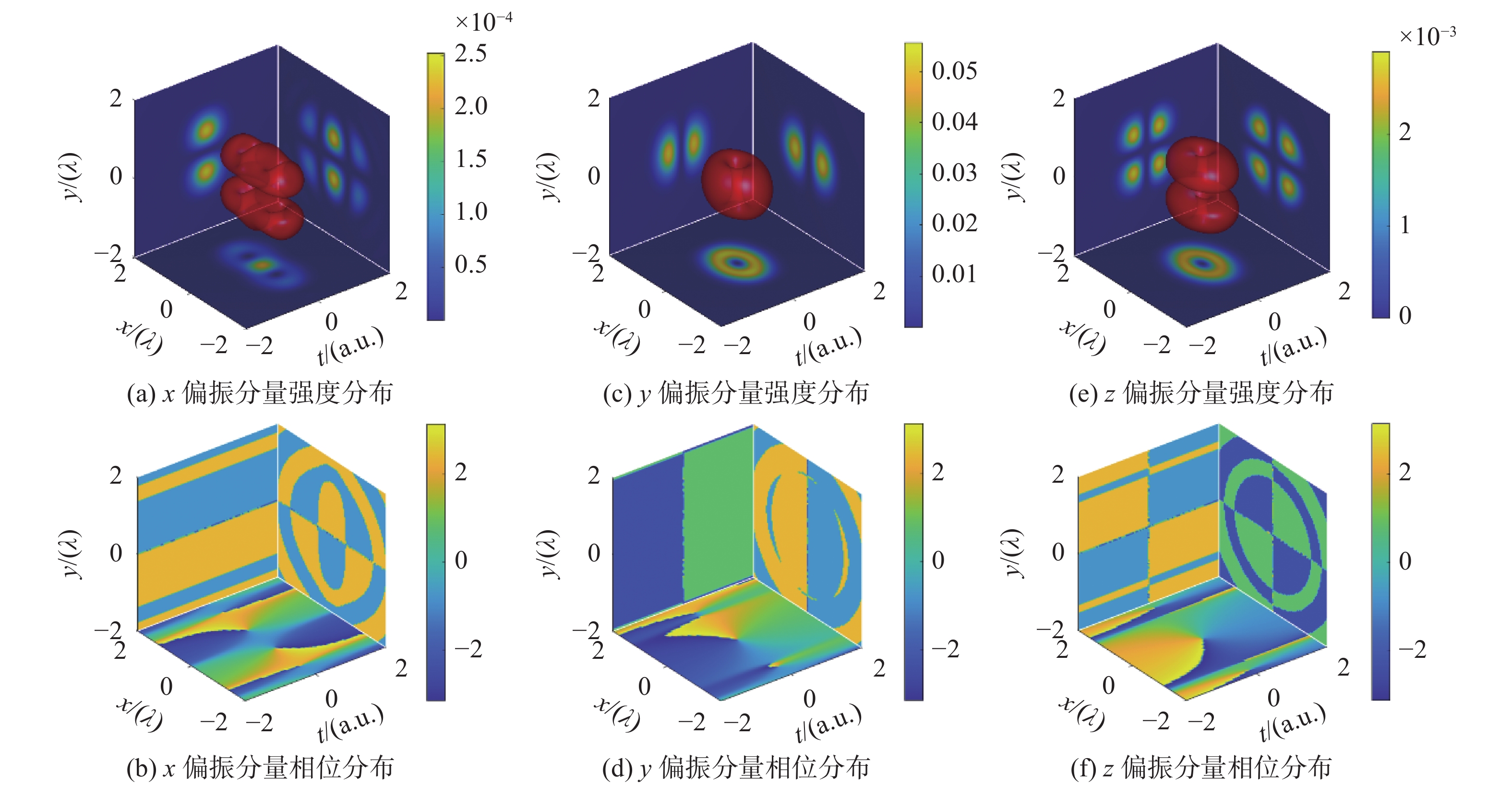
图7给出了垂直线偏振入射波包聚焦后焦场的x、y和z偏振分量的强度、相位以及等值面波包图(等值面为最大强度的20%)。从图7(a)可以看出x分量强度很小,比y分量低两个数量级,可以忽略不计。从图7(b)可以看出,x分量在x−t面内携带两个拓扑荷为+1的横向OAM。图7(c)显示聚焦波包的y分量有一个沿y轴的相位奇点轨迹,对应的相位分布如图7(d)所示,在x−t面从−π到π呈逆时针变化,这表明y分量携带拓扑荷为+1的横向OAM。从图7(e)可以看出聚焦时空涡旋具有较强的z分量。图7(f)显示z分量沿y轴有相位奇点轨迹,在x−t面的相位从−π到π呈逆时针变化,表明z分量携带一个拓扑荷为+1的横向OAM。
|
图 7 垂直线偏振焦场分量强度及相位图 Figure 7 Intensity and phase distribution of the vertically polarized focal field component |
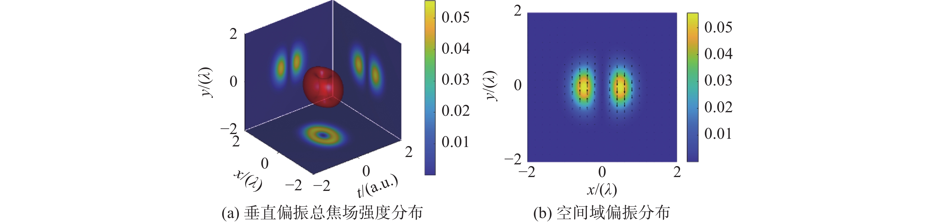
图8给出了聚焦时空涡旋的总强度和偏振分布。图8(a)为垂直线偏振总焦场强度分布及等值面波包图(等值面为最大强度的30%)。垂直线偏振总焦场波包形状与y分量基本一致。总焦场的波包形状由y分量决定。从图8(b) x−y面偏振分布图中可以看出聚焦波包在空间域的偏振分布为垂直线偏振。
|
图 8 垂直线偏振总焦场强度及x−y面偏振分布图 Figure 8 Total intensity and polarization distribution in x−y plane of vertically polarized STOV |
最后,图9给出了45°线偏振入射时空波包聚焦后焦场的x、y和z偏振分量的强度、相位以及等值面波包图(等值面为最大强度的20%)。从图9(a)、9(c)可以看到焦场的x分量和y分量的波包沿y轴都有一个相位奇点轨迹,观察图9(b)、9(d)可以发现x分量和y分量在x−t面有一个相位奇点,相位分布从−π到π呈逆时针变化,这表明他们都携带拓扑荷为+1的横向OAM。从图9(e)可以看出,聚焦时空涡旋的z分量峰值强度约为x分量的29%,其波包有两个倾斜的相位奇点轨迹;图9(f)显示z分量在x−t面有两个相位奇点,相位分布同样从−π到π呈逆时针变化,这表明z分量携带两个拓扑荷为+1的横向OAM。
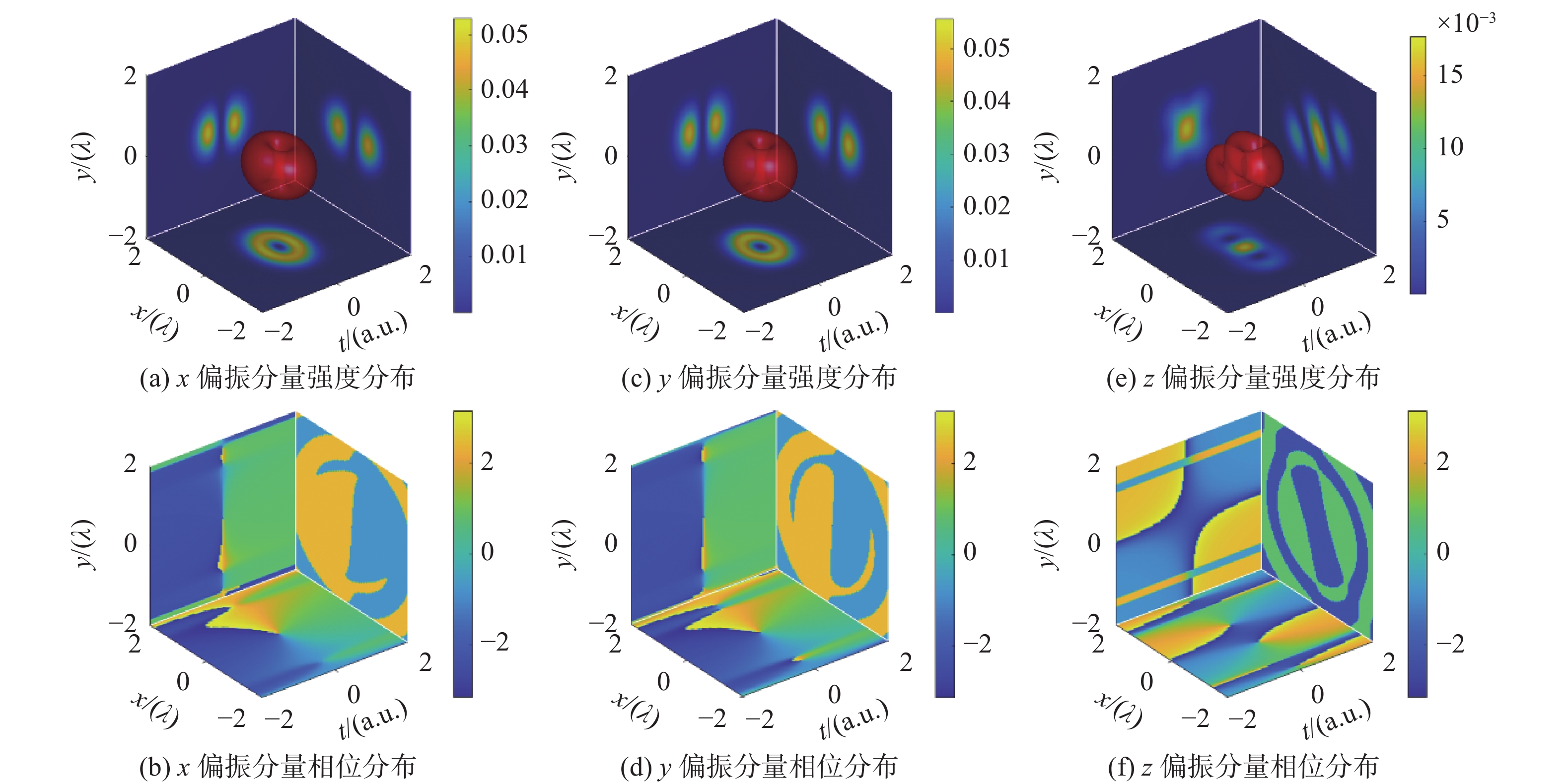
|
图 9 45°线偏振焦场分量强度及相位图 Figure 9 Intensity and phase distribution of 45° polarized focal field component |
图10给出了聚焦时空涡旋的总强度和偏振分布。图10(a)为总焦场强度分布及等值面波包图(等值面为最大强度的30%),可以看出波包中间的相位奇点轨迹不再是垂直于x−t面,其角度发生了一定的偏转。图10(b)清楚地显示聚焦场在空间域的偏振分布为45°方向线偏振。
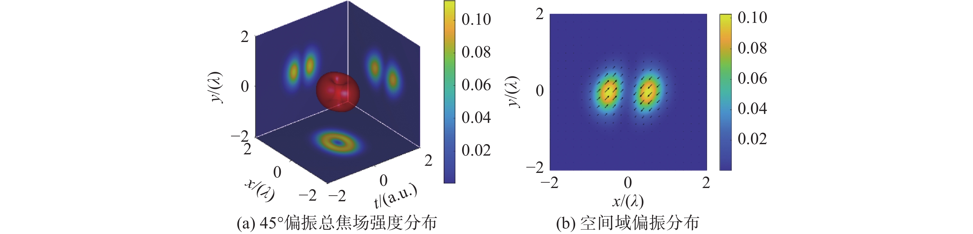
|
图 10 45°线偏振总焦场强度及x−y面偏振分布图 Figure 10 Total intensity and polarization distribution in x−y plane of 45° polarized STOV |
我们研究了预处理的线偏振波包经强聚焦生成具有横向OAM的时空光涡旋,并对其强度和相位分布特性进行了分析。水平线偏振入射波包强聚焦后,焦场主要由x偏振分量决定;垂直线偏振入射波包强聚焦后,焦场主要由y偏振分量决定;当45°偏振入射波包强聚焦后,焦场的水平偏振分量和垂直偏振分量强度基本相同,且均携带拓扑荷为+1的横向OAM。三种线偏振入射波包经高数值孔径透镜聚焦后,其焦场均具有较强的z分量;对于水平偏振和45°偏振入射波包而言,其强聚焦场的z分量具有两个横向相位奇点轨迹;对于垂直偏振入射波包而言,其强聚焦场的z分量则只有一个横向相位奇点轨迹。前期的研究在理论上生成了携带横向OAM的亚波长标量时空光涡旋,没有对焦场时空波包的偏振分析,本文将研究内容拓展到矢量场,加入针对线偏振特性的研究。报道的方法可以通过定制入射波包,经过高NA透镜聚焦后,在焦平面获得偏振态可控的具有横向OAM的高度局域线偏振时空光涡旋,其在光与物质相互作用、等离子体物理、光镊等方面有潜在的应用前景。
| [1] | ALLEN L, BEIJERSBERGEN M W, SPREEUW R J C, et al. Orbital angular momentum of light and the transformation of Laguerre-Gaussian laser modes[J]. Physical Review A, 1992, 45(11): 8185–8189. DOI:10.1103/PhysRevA.45.8185 |
| [2] | BETH R A. Mechanical detection and measurement of the angular momentum of light[J]. Physical Review, 1936, 50(2): 115–125. DOI:10.1103/PhysRev.50.115 |
| [3] | SIMPSON N B, DHOLAKIA K, ALLEN L, et al. Mechanical equivalence of spin and orbital angular momentum of light: an optical spanner[J]. Optics Letters, 1997, 22(1): 52–54. DOI:10.1364/OL.22.000052 |
| [4] | YAO A M, PADGETT M J. Orbital angular momentum: origins, behavior and applications[J]. Advances in Optics and Photonics, 2011, 3(2): 161–204. DOI:10.1364/AOP.3.000161 |
| [5] | MAIR A, VAZIRI A, WEIHS G, et al. Entanglement of the orbital angular momentum states of photons[J]. Nature, 2001, 412(6844): 313–316. DOI:10.1038/35085529 |
| [6] | UCHIDA M, TONOMURA A. Generation of electron beams carrying orbital angular momentum[J]. Nature, 2010, 464(7289): 737–739. DOI:10.1038/nature08904 |
| [7] | WANG J, YANG J Y, FAZAL I M, et al. Terabit free-space data transmission employing orbital angular momentum multiplexing[J]. Nature Photonics, 2012, 6(7): 488–496. DOI:10.1038/nphoton.2012.138 |
| [8] | BOZINOVIC N, YUE Y, REN Y X, et al. Terabit-scale orbital angular momentum mode division multiplexing in fibers[J]. Science, 2013, 340(6140): 1545–1548. DOI:10.1126/science.1237861 |
| [9] | BLIOKH K Y, NORI F. Spatiotemporal vortex beams and angular momentum[J]. Physical Review A, 2012, 86(3): 033824. DOI:10.1103/PhysRevA.86.033824 |
| [10] | JHAJJ N, LARKIN I, ROSENTHAL E W, et al. Spatiotemporal optical vortices[J]. Physical Review X, 2016, 6(3): 031037. DOI:10.1103/PhysRevX.6.031037 |
| [11] | HANCOCK S W, ZAHEDPOUR S, GOFFIN A, et al. Free-space propagation of spatiotemporal optical vortices[J]. Optica, 2019, 6(12): 1547–1553. DOI:10.1364/OPTICA.6.001547 |
| [12] | CHONG A, WAN C H, CHEN J, et al. Generation of spatiotemporal optical vortices with controllable transverse orbital angular momentum[J]. Nature Photonics, 2020, 14(6): 350–354. DOI:10.1038/s41566-020-0587-z |
| [13] | CHEN J, WAN C H, CHONG A, et al. Subwavelength focusing of a spatio-temporal wave packet with transverse orbital angular momentum[J]. Optics Express, 2020, 28(12): 18472–18478. DOI:10.1364/OE.394428 |
| [14] | BEIJERSBERGEN M W, ALLEN L, VAN DER VEEN H E L O, et al. Astigmatic laser mode converters and transfer of orbital angular momentum[J]. Optics Communications, 1993, 96: 123–132. |
| [15] | WOLF E. Electromagnetic diffraction in optical systems. I. An integral representation of the image field[J]. Proceedings of the Royal Society A: Mathematical, Physical and Engineering Sciences, 1959, 253(1274): 349–357. |
| [16] | RICHARDS B, WOLF E. Electromagnetic diffraction in optical systems. II. Structure of the image field in an aplanatic system[J]. Proceedings of the Royal Society A: Mathematical, Physical and Engineering Sciences, 1959, 253(1274): 358–379. |
| [17] | HELSETH L E. Focusing of atoms with strongly confined light potentials[J]. Optics Communications, 2002, 212: 343–352. |
| [18] | HELSETH L E. Optical vortices in focal regions[J]. Optics Communications, 2004, 229: 85–91. |